Showing posts sorted by relevance for query values. Sort by date Show all posts

Thursday, December 17, 2015

abortions on a cultural map

Inglehart–Welzel Cultural Map


Analysis of WVS data made by political scientists Ronald Inglehart and Christian Welzel asserts that there are two major dimensions of cross cultural variation in the world:

Traditional values versus Secular-rational values and Survival values versus Self-expression values. 

The global cultural map (below) shows how scores of societies are located on these two dimensions. Moving upward on this map reflects the shift from Traditional values to Secular-rational and moving rightward reflects the shift from Survival values to Self–expression values.

Traditional values emphasize the importance of religion, parent-child ties, deference to authority and traditional family values. People who embrace these values also reject divorce, abortion, euthanasia and suicide. These societies have high levels of national pride and a nationalistic outlook.

Secular-rational values have the opposite preferences to the traditional values. These societies place less emphasis on religion, traditional family values and authority. Divorce, abortion, euthanasia and suicide are seen as relatively acceptable. (Suicide is not necessarily more common.)

Survival values place emphasis on economic and physical security. It is linked with a relatively ethnocentric outlook and low levels of trust and tolerance.

Self-expression values give high priority to environmental protection, growing tolerance of foreigners, gays and lesbians and gender equality, and rising demands for participation in decision-making in economic and political life.

Cultural map - WVS wave 5 (2008)

Friday, November 6, 2015

P value and revalue

The P-Value controversy - What's a practitioner to do?


The recent controversy on p-values left many of us who work with data wondering what to do. Should we abandon p-values altogether and switch instead to reporting confidence intervals and effect sizes? Or should we go back to the basics and make sure we fully understand what p-values mean and how they should actually be applied?
тыцабельно

There are valid arguments to be made on both sides of the p-value divide. Assuming we still hold some faith in the goodness of the p-values, how do we re-calibrate our approach to using them?

First, we need to understand some of the history behind p-values in order to get some proper context. As clarified by Regina Nuzzo, the concept of p-value was introduced in the 1920's by Fisher "simply as an informal way to judge whether evidence was significant in the old-fashioned sense: worthy of a second look". However, over the years, p-values became the "bottom line" to a study (to borrow terminology employed by Steven Novella) - the end of the road rather than a promising beginning.

The notion of p-value as the "bottom line" for a study is interesting because it forces us to think about what needs to happen both before and after we draw that line.

Before we draw the "bottom line" for a study, we must remember that the p-value itself is an estimate, so its reliability will depend on a variety of factors, including an adequate study design, an appropriately selected sample, a set of validated and clean data collected from that sample, an appropriate statistical analysis for the research question of interest, a sufficiently large sample size, etc. This is what prompted Simonsohn to advise scientists to be transparent and "admit everything": how they determined their sample size, all data exclusions (if any), all data manipulations and all outcome measures used in the study . All of this information will provide a context for others to judge whether or not they can trust p-values reported in scientific publications.

After we draw the "bottom line" for a study, we need to bear in mind that the p-value requires us to make a decision and draw a conclusion: "Based on a p-value of 0.001 for our test, we decide to reject the null hypothesis Ho in favour of the alternative hypothesis Ha and we conclude that the data in our study provide strong evidence against the null hypothesis Ho." If we remember to focus on ourselves as agents responsible for making decisions and drawing conclusions based on evidence provided by the data, we will avoid the trap of believing we can play God and verify which of the null and alternative hypotheses is true. In 1925, Fisher himself claimed that the p-value indicates the strength of evidence against the null hypothesis. Years later, in 1955, he further claimed that "significance tests can falsify but never verify hypotheses".

If our data provide strong evidence against the null hypothesis Ho, we are in that promising situation where our findings are worthy of a second look. Something interesting may be going on and the only way to know whether this is the case is to try and replicate the findings of our study. We may be able to replicate these findings ourselves by conducting a second study or, most likely, others will get intrigued by our findings and proceed to conduct similar studies. In the latter situation, it is imperative for us to make it easy for others to replicate our study by adopting good practices advocated by proponents of reproducible research.

If our data fail to provide strong evidence against the null hypothesis Ho, we need to reflect on what may be at play (e.g., a sample size that was too small, a study design that was inadequate, a research question that needs to be refined, an outcome that needs to be reformulated, a fruitless research direction that needs to be aborted).

No study should be interpreted in isolation, just like no number (p-value included) should be interpreted in isolation

By

Isabella Ghement
по верхней ссылке диспут в линькедине

Wednesday, January 13, 2016

blood values

жопа хотел рашарить на фб, но:
The content you requested cannot be displayed right now. It may be temporarily unavailable, the link you clicked on may have expired, or you may not have permission to view this page.
вот и контент:

SPORTS
RUSSIAN ATHLETES ‘PUT IN DANGER’ BY DOPING PRACTICES, LEAKED IAAF LETTER REVEALS
BY TEDDY CUTLER ON 1/13/16 AT 10:54 AM

Russian athletes’ doping practices were so severe that the International Association of Athletics Federations (IAAF) feared they could die, leaked correspondence from 2009 reveals.

The Associated Press has published a letter dated October 14, 2009 from Pierre Weiss, who has been the IAAF’s general secretary since 2006, notifying Valentin Balakhnichev, then President of the All-Russia Athletics Federation (ARAF), of “startling” blood test results among the Russian athletes who competed at the 2009 Athletics World Championships in Berlin and the 2009 World Half Marathon Championships in Birmingham, England.

Balakhnichev was banned from the sport for life last week, along with Papa Massata Diack—the son of former IAAF president Lamine Diack—and IAAF treasurer Alexei Melnikov, for their parts in attempting to extort money from Russian marathon runner Liliya Shobukhova in return for covering up irregularities in her biological passport.

“Of the top 10 blood values recorded in Berlin, eight of them came from Russian athletes and many more than just these eight were also very suspicious,” the letter reads.

“In addition (and now not surprisingly) the blood values of the Russian athletes in Birmingham were also high, with three of the five athletes tested recording very suspicious values.

“These results are startling because not only are these athletes cheating their fellow competitors but at these levels are putting their health and even their own lives in very serious danger.”

The revelation that the IAAF was aware of the potential scale of Russian doping as far back as 2009 is another blow to the organization, the day before the publication of the World Anti-Doping Agency’s second report from its investigation into alleged IAAF corruption and Russian doping.

The first part of the report, published in November 2015, led to the indefinite suspension of Russia from athletic competition.

а узнать хотел:   что такое blood values ?


Wednesday, March 5, 2025

Walesa

After the US decision to suspend supplies to Ukraine, if the answer was in my gesture it would be "Let's do our part" not a step back. AMEN.

This is the text we signed:

Your Excellency Mr President,

We watched the report of your conversation with the President of Ukraine Volodymyr Zelenski with fear and distaste. We consider your expectations to show respect and gratitude for the material help provided by the United States fighting Russia to Ukraine insulting. Gratitude is due to the heroic Ukrainian soldiers who shed their blood in defense of the values of the free world. They have been dying on the frontline for more than 11 years in the name of these values and independence of their Homeland, which was attacked by Putin's Russia.

We do not understand how the leader of a country that is the symbol of the free world cannot see it.

Our panic was also caused by the fact that the atmosphere in the Oval Office during this conversation reminded us of one we remember well from Security Service interrogations and from the debate rooms in Communist courts. Prosecutors and judges at the behest of the all-powerful communist political police also explained to us that they hold all the cards and we hold none. They demanded us to stop our business, arguing that thousands of innocent people suffer because of us. They deprived us of our freedoms and civil rights because we refused to cooperate with the government and our gratitude. We are shocked that Mr. President Volodymyr Zelenski treated in the same way.

The history of the 20th century shows that every time the United States wanted to keep its distance from democratic values and its European allies, it ended up being a threat to themselves. This was understood by President Woodrow Wilson, who decided to join the United States in World War I in 1917. President Franklin Delano Roosevelt understood this, deciding after the attack on Pearl Harbor in December 1941 that the war for the defense of America would be fought not only in the Pacific, but also in Europe, in alliance with the countries attacked by the Third Reich.

We remember that without President Ronald Reagan and American financial commitment it would not have been possible to bring the collapse of the Soviet Union empire. President Reagan was aware that millions of enslaved people were suffering in Soviet Russia and the countries it conquered, including thousands of political prisoners who paid for their sacrifice in defense of democratic values with freedom. His greatness was m. in. on the fact that he without hesitation called the USSR the "Empire of Evil" and gave it a decisive fight. We won, and the statue of President Ronald Reagan stands today in Warsaw vis a vis of the US embassy.

Mr. President, material aid - military and financial - cannot be equivalent to the blood shed in the name of independence and freedom of Ukraine, Europe, as well as the whole free world. Human life is priceless, its value cannot be measured with money. Gratitude is due to those who make the sacrifice of blood and freedom. It is obvious for us, the people of "Solidarity", former political prisoners of the communist regime serving Soviet Russia.

We are calling for the United States to withdraw from the guarantees it made with the Great Britain in the 1994 Budapest Memorandum, which recorded a direct obligation to defend the intact borders of Ukraine in exchange for giving up its nuclear weapons resources. These guarantees are unconditional: there is no word about treating such aid as an economic exchange.

    • Lech Wales, b. political prisoner, Solidarity leader, president of the Republic of Poland III
    • Mark Bailin, b. political prisoner, editor of independent publishing houses
    • Severn Blumstein, b. political prisoner, member of the Workers' Defense Committee
    • Teresa Bogucka, b. a political prisoner, activist of the democratic opposition and Solidarity
    • Gregory Bogut, b. political prisoner, activist of democratic opposition, independent publisher
    • Mark Borowik, b. political prisoner, independent publisher
    • Bogdan Borusewicz, b. political prisoner, leader of the underground Solidarity in Gdansk
    • Zbigniew Bujak, b. political prisoner, leader of the underground Solidarity in Warsaw
    • Władysław Frasyniuk, b. political prisoner, leader of the underground Solidarity in Wrocław
    • Andrew Gintzburg, b. a political prisoner, activist of the underground Solidarity
    • Richard Grabarczyk, b. a political prisoner, Solidarity activist
    • Alexander Janiszewski, b. a political prisoner, Solidarity activist
    • Peter Kapczy otrski, b. a political prisoner, activist of the democratic opposition
    • Mark Kossakowski, b. political prisoner, independent publicist
    • Christopher the King, b. a political prisoner , independence activist
    • Jaroslav Kurski, b. a political prisoner, activist of the democratic opposition
    • Barbara Swan, b. a political prisoner, activist of the underground Solidarity
    • Bogdan Lis, b. political prisoner, leader of the underground Solidarity in Gdansk
    • Henryk Majewski, b. a political prisoner, Solidarity activist
    • Adam Michnik, b. political prisoner, activist of the democratic opposition, editor of independent publishing houses
    • Slavomir Najniger, b. a political prisoner, activist of the underground Solidarity
    • Peter the German , b. political prisoner, journalist, and printer of underground publishing houses,
    • Stefan Konstanty Niesiołowski, b. a political prisoner , independence activist
    • Edward Nowak, b. a political prisoner, activist of the underground Solidarity
    • Wojciech Onyszkiewicz, b. political prisoner, member of the Workers' Defence Committee, Solidarity activist
    • Anthony Pawlak, b. a political prisoner, activist of the democratic opposition and underground Solidarity
    • Sylwia Poleska-Peryt, b. a political prisoner, activist of the democratic opposition
    • Christopher Push, b. a political prisoner, activist of the underground Solidarity
    • Richard Push, b. a political prisoner, activist of the underground Solidarity,
    • Jacek Rakowiecki, b. a political prisoner, activist of the underground Solidarity
    • Andrew Severn, b. political prisoner, actor, director of the Polish Theater in Warsaw
    • Witold Sielewicz, b. political prisoner, printer of independent publishing houses
    • Henryk Sikora, b. a political prisoner, Solidarity activist
    • Christopher Siemien Krski, b. political prisoner, journalist, and printer of underground publishing houses
    • Gra ,yna Staniszewska, b. a political prisoner, leaders of Solidarity of the Beskids region
    • George Degrees, b. a political prisoner, activist of the democratic opposition
    • Joanna Happy, b. political prisoner, editor of Solidarity underground press
    • Ludwik Turko, b. a political prisoner, activist of the underground Solidarity
    • Matthew Wierzbicki, b. political prisoner, printer and publicist of independent publishing houses

Monday, December 12, 2022

Ecological Values of the Population of Belarus: Theoretical and Empirical Levels

Экологические ценности населения Республики Беларусь: теоретический и эмпирический уровни.

Социологический альманах. Вып.4. С.352-363.


The author discusses the ecological values of the population of Belarus that have been measured empirically on the level of mass consciousness and mass behavior. The empirical results have been compared with the theoretical model of ecological values that fits the sustainable development model of societal development. Special attention is paid to the actual level of ecological awareness of the population that currently does not actively stimulate ecologically oriented behavior.

Keywords: 

ecological values, ecological consciousness, ecological behavior, ecological awareness, Belarus. 


Wednesday, September 25, 2024

Europe’s COVID-19 death toll in 2020 and 2021: stark regional differences September 2, 2024

By Florian Bonnet, Pavel Grigoriev, Markus Sauerberg, Ina Alliger, Michael Mühlichen and Carlo-Giovanni Camarda

Europe was hard-hit by the COVID-19 pandemic in 2020 and 2021. While its effects at national level are now well known, intranational differences have been less frequently investigated. Florian Bonnet, Pavel Grigoriev, Markus Sauerberg, Ina Alliger, Michael Mühlichen and Carlo-Giovanni Camarda fill this knowledge gap and show that considerable heterogeneity exists at regional level, even within the same country.


In 2020 and 2021, drastic measures were taken to combat the COVID-19 pandemic, contain the spread of the virus and limit the number of deaths. The efficacy of these measures, initially hard to evaluate (Caporali et al 2022), can be better assessed today, as reliable estimates of deaths caused by this pandemic are now being published by major research institutes in scientific journals and by international organizations. In a report issued in May 2024, for instance, the World Health Organization (WHO) estimated that life expectancy dropped by 1.8 years between 2019 and 2021 globally, erasing a decade of progress.

COVID-19-related excess mortality


These estimates are derived from what is known as excess mortality, which represents the difference between observed mortality during the pandemic years and the mortality that would have been expected in its absence. Excess mortality can be quantified using different indicators, such as the number of excess deaths. However, comparing this indicator between countries of different sizes and age structures can be misleading. Another informative metric is the loss of life expectancy at birth, calculated globally by organizations like WHO.

The regular calculation, publication, and dissemination of excess mortality indicators serve as crucial tools for comparing the pandemic’s impact across different countries at national level. However, the pandemic did not have a homogeneous impact at subnational level, primarily due to the varying confinement strategies implemented to curb the spread of the virus. This variability underscores the importance of quantifying these indicators at a more granular geographical level to highlight the pandemic’s impact in the regions most severely affected. Detailed geographical analysis of excess mortality can thus localize the effect of the pandemic and help tailor response strategies accordingly.

Mortality in Europe at subnational level: 2020 and 2021


In a series of studies published in 2024, we first proposed an innovative method to calculate excess mortality at a fine regional level (Bonnet and Camarda 2024), then used this method to estimate the levels of excess mortality in 561 European regions covering 21 countries in 2020 (Bonnet et al 2024a). We finally expanded our geographical scope to 569 regions covering 25 European countries, differentiating between the two pandemic years, 2020 and 2021 (Bonnet et al. 2024b). These estimates are the outcome of a thorough process involving the collection of data from a wide array of national statistical institutes. Here, we present our findings based on loss of life expectancy at birth for both sexes combined.
Figure 1 depicts the spatial distribution of the estimated life expectancy losses in 2020. Losses were highest in northern Italy and central Spain, with values close to 4 years in the regions of Bergamo and Cremona, 3.5 years in Piacenza, and 3 years in the Spanish regions of Segovia, Ciudad Real, Cuenca, and Madrid. They are even higher when considering only men (not shown here), who were more severely affected by the pandemic: life expectancy loss is close to 5 years in Cremona and 4.5 years in Bergamo. Losses in 2020 were more moderate, though still dramatic, in eastern Europe (notably in Poland), eastern Sweden, and northern and eastern France. In the latter, the Paris region and areas near the German border showed the highest values, ranging from 1.5 to 2 years. Conversely, the losses were much lower in other geographical areas, such as southern Italy, much of Scandinavia and Germany, and western France, where life expectancy remained close to what would have been expected in the absence of the pandemic.

Figure 2 presents the estimated life expectancy losses in 2021. At first glance, the regions affected by excess mortality were not the same as in 2020. The most significant losses were predominantly in eastern Europe. More broadly, among the regions where life expectancy losses exceed 2 years, we find 61 of the 73 Polish regions, 12 of the 14 Czech regions, all eight Hungarian regions, seven of the eight Slovak regions, but only one Italian region and one Spanish region, even though these two countries were also heavily impacted in 2020. Moreover, the life expectancy losses were much greater in Germany in 2021 than in 2020, especially in the eastern part of the country where values often exceed 1.5 years. In southern Saxony, Halle, and Lusatia, losses were nearly 2 years. Conversely, the lowest values were observed in Spain and Scandinavia. In France, life expectancy losses were more uniform than in 2020, generally ranging between 0 and 1.5 years, with the highest loss in the Parisian 
suburbs (Seine-Saint-Denis) where it reached 1.5 years (2 years for men).

Ranking European regions


Combining the data from both years, an overall assessment of the mortality impact of COVID-19 is possible (Bonnet et al 2024b). The regions where mortality increased the most in 2020 and 2021 are Pulawy, Bytom, and Przemyski in south-eastern Poland, and Kosice and Presov in eastern Slovakia. More broadly, eastern European regions predominate among the top 50 regions, which include 36 Polish regions, six Slovak regions, two Czech regions, one Hungarian region, and the two Lithuanian regions. Notably, the Italian regions of Cremona, Bergamo, and Piacenza complete this panel, ranging between the 15th and 30th places. In France, Seine-Saint-Denis ranks 81st, while all other French regions rank below the 100th place.

Conclusions


In conclusion, analyzing the impact of a crisis like the COVID-19 pandemic on longevity at a fine geographical scale is essential, as within-country disparities can be significant. This was notably true for Italy in 2020 (between the South and the North), and for Germany in 2021 (between the west and the east). Our study highlighted the severe impact of the pandemic in certain European regions, where the loss of life expectancy exceeded 3 years. The most affected regions shifted between 2020 and 2021, moving from areas with traditionally high life expectancy (northern Italy, central Spain, Greater Paris) to those with traditionally low life expectancy (Eastern Europe). France was relatively spared compared to the rest of Europe except for Seine-Saint-Denis. The coming years will be crucial for determining whether life expectancy levels return to their long-term trajectory or whether the pandemic has caused a structural impact in certain regions.

References

  • Caporali, A., Garcia, J., Couppié, É., Poniakina, S., Barbieri, M., Bonnet, F., … & Torres, C. (2022). The demography of COVID-19 deaths database, a gateway to well-documented international data. Scientific Data, 9(1), 93.
  • Bonnet, F., & Camarda, C. G. (2024). Estimating subnational excess mortality in times of pandemic. An application to French départements in 2020. PLoS ONE, 19(1), e 0293752.
  • Bonnet, F., Grigoriev, P., Sauerberg, M., Alliger, I., Mühlichen, M., & Camarda, C. G. (2024a). Spatial variation in excess mortality across Europe: a cross-sectional study of 561 regions in 21 countries. Journal of Epidemiology and Global Health, 1-10.
  • Bonnet, F., Grigoriev, P., Sauerberg, M., Alliger, I., Mühlichen, M., & Camarda, C. G. (2024b). Spatial disparities in the mortality burden of the covid-19 pandemic across 569 European regions (2020-2021). Nature Communications, 15(1), 4246.

Thursday, July 15, 2021

Average length of life spent childless

Cross-sectionally speaking

July 12, 2021 Ryohei Mogi, Jessica Nisén and Vladimir Canudas-Romo
O!
In addition to the commonly used fertility measures, Ryohei Mogi, Jessica Nisén, and Vladimir Canudas-Romo suggest an alternative approach to the study of first birth behaviour, focusing on how long women live childless. A visual decomposition analysis shows how different cohorts contribute to cross-country differences in the length of childless life.

Postponement (Kohler et al. 2002) and foregoing (Kreyenfeld and Konietzka 2017) of parenthood have been important family demographic trends of the past half-century in the developed world. The common indexes used to describe first birth patterns (such as age-specific first birth rates, mean age at first birth, proportion of women remaining childless), tend to focus on a specific dimension (timing or quantum) but risk losing sight of the general picture. We propose an alternative measure, the cross-sectional average length of life childless, or CALC (Mogi et al. 2021).

How many of their reproductive years do women spend childless?


Table 1 shows CALC in 2015 in 11 selected countries where CALC tends to be high, frequently representing more than half of a woman’s reproductive life (between ages 12 and 49), i.e. more than 19 years. Japan and Spain record the highest values: in 2015, women in these countries spent, on average, almost 60 per cent of their reproductive lives without children (23.2 and 22.5 years in Japan and Spain, respectively). In Czechia, Denmark, Hungary, the Netherlands, and Sweden, CALC ranges between 19.2 and 20.9 years. Sweden lies in the middle, at 19.8 years. The lowest values are found in Belarus and the United States, where women remain childless for 16.0 and 17.5 years, respectively.
These examples clearly illustrate that CALC may reflect trends in both timing and quantum of first births. For instance, Japan and Spain are characterized by both late timing of first births as well as high levels of lifetime childlessness, while early timing and low levels of lifetime childlessness are common in Belarus and the United States.

Contribution of ages and cohorts to the difference in CALC


Japan

Using Sweden (median value) as a standard of reference, we can better appreciate how ages and cohorts contribute to high or low values of our index (CALC) in three selected cases: Hungary, Japan, and the United States (see also the interactive online application: https://rmogi.shinyapps.io/CALC/).

Sweden, our country of reference, is characterized by moderate levels of lifetime childlessness, and average-to-late timing of first births, with a notable catch-up at higher ages (Andersson et al. 2009, Kreyenfeld and Konietzka 2017). Compared to their Swedish counterparts, Japanese women have a greater risk of being childless across all reproductive ages and cohorts, and their CALC was particularly high in 2015 (Figure 1). Younger cohorts of women in Japan are contributing to an even higher expectation of childless life from increasingly early ages, probably a reflection of their later marriage and lower marriage rates (NIPSSR 2019).

United States

The decomposition of the difference in CALC between the United States and Sweden reflects the impact of high first birth rates at young ages in the United States and the catching-up process of childbearing in Sweden at later ages (at least among women born between the late 1960s and mid-1970s; Figure 2). In the younger cohorts, born in the mid-1970s or later, there are indications that the subgroup difference in life spent without children at reproductive ages in the United States is intensifying. Indeed, there is significant variation in first birth behaviour by race/ethnicity in the United States, because Hispanic white and Non-Hispanic African American women continue to enter motherhood earlier than Non-Hispanic white women (Sullivan 2005).
Hungary

Finally, the decomposition of the difference in CALC between Hungary and Sweden is particularly interesting because it shows how different cohorts may be affected simultaneously at different ages, contrasting period and cohort effects on first births. In this case, the period effect occurs in the years following the onset of the Great Recession in 2007, which strongly affected fertility rates in many Central and Eastern European countries (Matysiak et al. 2020), and it seems probable that the recession is contributing to a longer expectation of childless life at reproductive ages in Hungary than in Sweden.

Concluding remarks


To conclude, CALC is a newly introduced measure that applies core demographic life table methodology to first births, shedding light on first birth patterns and trends and related cross-country differences. Further, visualization of the decomposition of differences between two CALCs provides a tool for illustrating how different cohorts and ages contribute to cross-country differences in the length of life childless during reproductive ages. This characteristic of CALC may be useful for policymakers, for instance, because specific population subgroups still in their reproductive ages may be identified and targeted, if considered necessary.

References

  • Kohler, H. P., Billari, F. C., & Ortega, J. A. (2002). The emergence of lowest-low fertility in Europe during the 1990s. Population and Development Review, 28(4), 641–680.Kreyenfeld, M., & Konietzka, D. (2017). Childlessness in Europe: Contexts, Causes, and Consequences. Springer.
  • Matysiak, A., Sobotka, T., & Vignoli, D. (2020). The Great Recession and fertility in Europe: A sub-national analysis. European Journal of Population, 37, 29­–64.
  • Mogi, R., Nisén, J., & Canudas-Romo, V. (2021). Cross-sectional average length of life childless. Demography, 58(1), 321–344.
  • National Institute of Population and Social Security Research (2019). Recent demographic statistics. National Institute of Population and Social Security Research [in Japanese].
  • Sullivan, R. (2005). The age pattern of first-birth rates among U.S women: The bimodel 1990s. Demography, 42(2), 259–273.

Wednesday, August 2, 2017

causes amenable to personal health care

это насколько понимаю самолечение
мб, кто-то под правит, потому что доступность
Map of HAQ Index values, by decile, in 1990 (A) and 2015 (B)

Map of HAQ Index values, by decile, in 1990 (A) and 2015 (B) 

Deciles were based on the distribution of HAQ Index values in 2015 and then were applied for 1990. HAQ Index = Healthcare Access and Quality Index. ATG=Antigua and Barbuda. VCT=Saint Vincent and the Grenadines. LCA=Saint Lucia. TTO=Trinidad and Tobago. TLS=Timor-Leste. FSM=Federated States of Micronesia.

см подробнее

Healthcare Access and Quality Index based on mortality from causes amenable to personal health care in 195 countries and territories, 1990–2015: a novel analysis from the Global Burden of Disease Study 2015

Friday, July 7, 2023

The new Asian family

East Asian governments must try to manage a momentous social change they cannot prevent

насколько мы востчные? думаю: да, география мало что меняет

The concept of “Asian values”, once championed by leaders across the region, went out of vogue after the Asian financial crisis of 1997. The idea that East and South-East Asia’s disciplined governments had a unique economic edge over the decadent West suddenly seemed less compelling. Today in prosperous East Asia a different facet of those ballyhooed values is looking even more parlous. In China, Japan, South Korea and Taiwan, Asians’ supposed commitment to conservative family life is collapsing. As we report in our Asia and China sections this week, millions of young people are opting for looser, often lonelier and—in the East Asian context—less male-dominated arrangements. In a region that is home to over a fifth of humanity, the socioeconomic and demographic consequences will be vast, potentially destabilising and will shape millions of lives.

In Japan, where the shift first became evident, married couples with at least one child accounted for 42% of households in 1980, and single people 20%. That has flipped. In 2020 couples with children accounted for 25% of households, and singletons 38%. And the decline is continuing. Last year 17% of Japanese men and 15% of women aged 18-34 said they would not marry, up from 2% and 4% in the early 1980s, and China recorded its lowest-ever number of marriages, half as many as a decade ago.

In some ways young Chinese, Japanese, Taiwanese and South Koreans are following a path charted in rich countries elsewhere. Between 1960 and 2010 Europe’s marriage rate fell by half, for many of the reasons that are now driving down East Asian rates. To many people, marriage seems increasingly anachronistic and unaffordable. Across East Asia it is still widely understood in Confucian terms, as the union of a dominant man and submissive woman. In South Korea a married woman is referred to as Jip-saram, or “home person”, and her husband as Bakat-yangban, or “man outside”.

High property prices are an added disincentive to setting up a marital home. Alternative domestic arrangements are becoming more accepted; besides singledom, they include intergenerational flat-sharing and, less often, cohabiting and gay partnerships. And growing numbers of middle-class women are putting off marriage to concentrate on their careers.

Traditional values are hard on women at work, too. East Asia has some of the world’s best-educated women, yet its overall record on female empowerment is poor and in some ways worsening. On the World Economic Forum’s gender-equality ranking of 153 countries, China—where women are said to “hold up half the sky”—slipped from 63rd in 2006 to 102nd in 2022. South Korea has the widest gender pay gap in the oecd.

If most of this sounds familiar, two things make East Asia’s great social change distinct and hugely troublesome. First, the taboo against having children outside marriage remains as rigid as ever. Across the oecd, 40% of births are outside wedlock. In Japan, South Korea and Taiwan less than 5% are. (The figure in China is unavailable, revealingly, but not thought to be higher.)

The result is a plummeting fertility rate. South Korea’s, at 0.78, is the lowest recorded anywhere and Taiwan’s only slightly higher. Japan’s and China’s are just above half the replacement rate. China’s cruel one-child policy, now replaced by panicked officials with calls to have three, exacerbated its demographic squeeze. But as the regional picture shows, it would have happened anyway. The total population of the four East Asian countries is predicted to shrink by 28% between 2020 and 2075.

The second problem is that the region’s governments are making the situation worse. None seriously broaches the only policy guaranteed to revive East Asia’s flagging demography: mass immigration. Their main response is to try to resuscitate marriage with economic perks—including tax breaks and subsidised weddings—with little success. South Korea’s president, Yoon Suk-yeol, admits that his country has, in essence, squandered 280trn won ($215bn) on such policies. Worse, he and his counterparts in China and Japan are doubling down on the conservative approach that their citizens increasingly object to.

South Korea’s previous administration sought to extend benefits to single parents and unmarried couples. Mr Yoon, who blames the low fertility rate on feminism, has put a stop to that. Under Xi Jinping, China promises its citizens a Confucian revival and arrests gay-rights activists. Japan’s ever-ruling Liberal Democratic Party is also against reforming marriage, including by refusing to make it available to gay couples, although most voters want to see that change.

There are pockets of progress, notably in Taiwan, which recently took a more liberal course. It has legalised same-sex marriage and in May permitted gay couples to adopt children—though it is too soon to know whether these changes will show up in the statistics. But the region as a whole is stuck between modernity and tradition, suffering some of the worst effects of both. East Asians are free to disdain traditional family roles, but not to redefine them. That is why millions resort to childlessness and solitude.

Governments should try to complete this lopsided revolution. Even if social change is not entirely within their grasp, and does not happen overnight, they can at least stop resisting it. To make family life more attractive, they need to deal with its gender imbalances as well as its costs by, for example, making paternity leave routine. They should look beyond heterosexual marriage, as their citizens have, and extend legal recognition to cohabiting, gay and other non-traditional arrangements—and afford them the support married couples now enjoy, especially over child-rearing. It is self-defeating and outrageous that China prevents single women from freezing their eggs, or that Japan makes it nearly impossible for gay couples to foster children.

Let them not wed


Such policies would not fix the region’s demography. But they would have a more positive effect on it than the current ones. More important, they would leave millions freer to lead the lives they choose, especially women and gay people. East Asian governments have overseen the greatest-ever economic boom. Now they must attend to their citizens’ happiness and liberty. ■

For subscribers only: to see how we design each week’s cover, sign up to our weekly Cover Story newsletter.

This article appeared in the Leaders section of the print edition under the headline "The new Asian family"

Monday, April 26, 2021

MARRIAGE COUNTERFACTUALS IN JAPAN

VARIATION BY GENDER, MARITAL STATUS, AND TIME


Family demographers have long been interested in the debate surrounding changes in the marriage institution, associated with concepts such as the deinstitutionalization of marriage and the Second Demographic Transition. These perspectives focus on alternatives to traditional heterosexual marriage (what can be termed the external context of marriage), such as lifetime singlehood, same-sex marriage, and non-marital cohabitation. In research co-authored with Erik Bond and Ann Beutel, recently published in Demographic Research, we take a different perspective on this debate by focusing on what we term the internal context of marriage, or how social, economic, psychological, and personal dimensions of the marriage experience are perceived by relevant stakeholders (i.e., men and women, comparing those currently married vs. never married).

Using cross-sectional Japanese data from the 1994 National Survey on Work and Family Life and the 2000 and 2009 National Survey of Family and Economic Conditions (NSFEC) (combined N = 8,467), we construct unique measures of this internal context, which we call “marriage counterfactuals”. These measures gauge how people perceive that marriage, or the lack thereof, may have altered their lives.

Why Japan?


Japan is an interesting setting for several reasons. Being the first non-Western country to industrialize, it experienced many of the same economic changes and some similar demographic changes as those in the West (e.g., increasing delays in marriage and rates of lifetime singlehood). However, unlike Western countries, Japan witnessed limited changes in some other social spheres. One notable example here is the family sphere – engagement in alternatives to traditional marriage remains rather culturally limited or legally unavailable (as in the case of same-sex marriage).

Japan is also an interesting setting because it maintains a highly gendered division of household labor within marriage, with men still playing the role of intensive breadwinner and women the role of homemaker. Starting in the 1990s, a time period covered by our data, the Japanese economy experienced a significant downturn and prolonged recession. Ensuing changes in the labor market made it difficult for young men to find suitable employment to realize the breadwinner role.

Because marriage and fertility in Japan are closely related, failure to realize marital intentions is concomitantly linked to failure to meet fertility intentions. Having a fertility rate that is well below replacement level for many decades, and facing the reality of having one of the oldest population age structures in the world has significant implications for Japan’s demographic future. Thus, understanding how relevant stakeholders perceive marriage in Japan’s marriage market (especially during a period of considerable economic change and labor market restructuring) is of considerable interest.

Analytical Strategy for the Study


Our sample consisted of people aged 20 to 49. The marriage counterfactual measures used for our study came from a series of survey items that asked respondents to indicate how they perceived that their life would be different (on five dimensions, captured by separate survey items) if they had a marital status that differed from the one they held at the time of the survey. These items concerned change in dimensions such as social respect, emotional security, living standard, freedom, and overall satisfaction. Specifically, married respondents were asked to imagine their life (on the above dimensions) if they had gone unmarried. Non-married respondents, in turn, were to imagine what it would be like to be married. Previously-married respondents were not used in the analysis as they were not asked these questions.

These variables were measured on a 5-point Likert scale, with the following categories: “Much Worse,” “Somewhat Worse,” “Same,” “Somewhat Better,” and “Much Better.” To facilitate the analysis of the pooled data, we coded the variables so that higher values indicate that married life is viewed more as a benefit than single life, and lower values indicate the reverse (that married life is viewed more as a cost than single life). To avoid awkward phrasing, as a shorthand, we use terminology related to the idea of “benefits of marriage” to describe our results.

Findings Related to Marriage Counterfactuals


Figures 1 through 3 show the distribution of marriage counterfactual measures for, respectively, the full sample, by marital status, and by gender.

For the entire sample (Figure 1), as well as across marital statuses and genders, respondents generally perceived ’emotional security’ and ‘overall satisfaction’ as benefits of being married, ‘personal freedom’ as a cost of being married, and ‘respect from others’ as unaffected by marriage. Compared to never-married respondents, currently married respondents were more likely to see ‘living standard’ as a marriage benefit (Figure 2). In comparison to women (Figure 3), men were more apt to view ‘respect’ and ‘emotional security’ as marriage benefits, while women perceived ‘standard of living’ as more of a benefit (consistent with the prevalence of the man-as-breadwinner/woman-as-homemaker household division of labor and the Japanese labor market’s general discriminatory environment toward women).

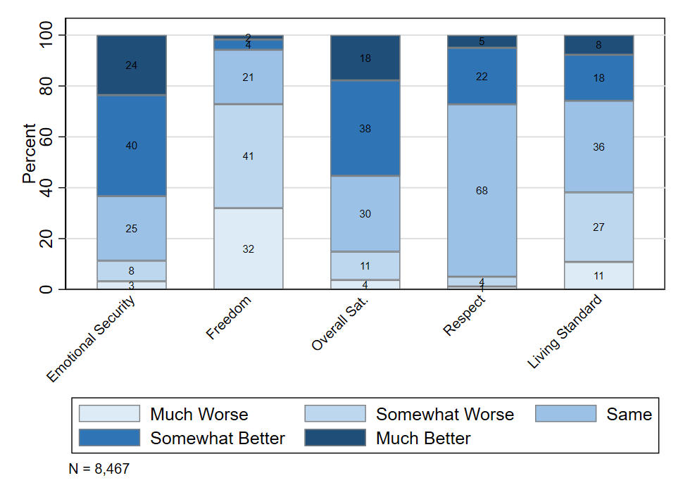
Figure 1. Distribution of Counterfactual Marriage Measures

Figure 2. Distribution of Marriage Counterfactual Measures by Marital Status

Figure 3. Distribution of Marriage Counterfactual Measures by Gender

Logistic Regression Analysis


We also conducted a series of ordered logistic regression models to examine the determinants of the marriage counterfactual measures, the dependent variables in our analysis. The main independent variables of interest were measures of gender, marital status, and time period; we also controlled for education, employment status, urban upbringing, and home-ownership. We estimated models for the pooled sample as well as separate models by gender and by marital status. More detailed results are available in the article version of our research.

Our main findings were that perceptions of the marital benefits worsened over time. This is consistent with deteriorating economic conditions and the general assertion that marriage and work/the division of labor are deeply connected in Japanese society. Furthermore, never-married respondents tended to view marriage in more favorable terms than their married counterparts (particularly with regard to freedom and respect from others). Finally, with the exception of the standard of living dimension, men viewed marriage benefits more favorably than women. However, to our surprise considering the man-as-breadwinner role, we find that both men and women viewed marriage benefits less favorably. This may be a result of the general worsening of the marriage market in Japan related to the deteriorating economic situation or to rising income among single women.

Conclusions


Based on our research, we end with four concluding thoughts.

First, despite some dimensions of marriage continuing to be viewed in favorable terms, the key change is that marriage benefits are being viewed less positively over time. In conjunction with other research on family-related attitudes in Japan, this suggests that ideas about marriage there are experiencing substantive change. Thus, it is especially important to consider, as we have, the marital perceptions not only of those who are already married, but also of those who will shape the future of the institution: the not-yet-married.

Second, the internal context of marriage – perceptions of standard of living, respect from others, emotional security, freedom, and overall satisfaction – are important and generally overlooked aspects of the marriage institution. The focus on the external context of marriage and the preoccupation with marriage deinstitutionalization, as well as diversity in family forms, largely ignores these factors, giving an incomplete picture of changes in modern marriage.

Third, gender differences in our analysis make it clear that the traditional division of household labor (i.e., the man-as-breadwinner/woman-as-homemaker model) continues to be influential in Japan.

Fourth, relatedly, in spite of structural changes to the economy and labor market, cultural beliefs regarding traditional marriage persist. We wonder whether this situation will continue or whether, conversely, new partnership forms will begin to gain ground in Japan, a place where such alternatives currently go against the cultural grain.

Authres' Short Bio


Martin Piotrowski is an Associate Professor of Sociology at the University of Oklahoma. He received his PhD in sociology from the University of North Carolina at Chapel Hill and was trained at the Carolina Population Center (CPC). His research focuses on aspects of rural-to-urban migration, marriage and fertility, and familial and gender attitudes especially in parts of Asia and most recently parts of Europe. He has done research in several countries including Thailand, Nepal, China, Japan, and Poland and has explored topics involving inter-generational and family relations, household structures, and life course transitions. He has published widely in sociology, family, and demography journals.

Erik Bond is an Assistant Professor of Sociology at Miyazaki International College. He received his PhD in sociology from the University of Oklahoma. His research has focused on marital and gender attitudes in Japan and international-comparative contexts, particularly as they interplay with macro cultural, labor, and policy regimes over time. He has special interest in the use of novel statistical methods for revealing latent values in large data sets. He also works as an LGBTQ+ and diversity advocate in southern Japan.

Ann M. Beutel is an Associate Professor of Sociology at the University of Oklahoma. She received her PhD in sociology from the University of Minnesota. Her research has focused on the influence of social location on values, attitudes, and expectations of adolescents and adults and on the relationship between gender and experiences in education and the labor market. She has carried out her research using data from a number of countries, including the United States, Nepal, South Africa, and Japan.

Sunday, December 29, 2019

The significance of age to the study of ethnic residential segregation

Published on N-IUSSP.ORG October 29, 2018

L'importance de l'âge dans l'étude de la ségrégation résidentielle ethnique


Albert Sabater, Gemma Catney

In the study of ethnic residential segregation, global measures are typically used. However, while useful as summary indicators, these measures miss important and distinctive age-specific and birth-cohort trends. Albert Sabater and Gemma Catney demonstrate this for England and Wales (2001 and 2011).

Are there distinctive patterns of ethnic residential segregation across the life course?


In a recent publication (Sabater and Catney 2018), we examine variations in ethnic residential segregation across the life course, represented in our study by particular age groups and ‘stages’ of life. We argue that taking such an approach is important in contexts with the simultaneous growth of young and aging minority ethnic populations for understanding the local dynamics of ethnic geographies.

Using harmonized small area data (8,546 wards) for England and Wales (2001-2011), we demonstrate the usefulness of our approach by applying two measures of segregation: the dissimilarity index (ID) and the isolation index (P*). These two commonly-employed measures capture two key dimensions of residential segregation (evenness and exposure) and allow straightforward comparisons of global, age group and birth-cohort segregation both nationally and internationally. In the study, we analyze the evolution of ethnic residential geographies for the eight largest and most stable categories from 2001 to 2011: White British, Other White, Indian, Pakistani, Bangladeshi, Black Caribbean, Black African and Chinese. Ethnicity data used in UK national statistics relies on individuals’ self-definition.

The computation of ethnic residential segregation with an age dimension is equivalent to the summary or ‘global’ calculation for all groups, although the analysis relies on an index value for each age group. The use of age for the analysis of ethnic residential segregation increases our knowledge about the spatial incorporation of each group because it highlights two important characteristics about an individual: their place in the life cycle – whether a young adult, middle-aged or older – and their membership in a cohort of individuals who were born at a similar time. Further, since the characteristics of younger or older adults may differ at a given period, the use of birth-cohorts provides one way to examine the trajectory of residential segregation of ethnic groups as they pass through life-course phases, including when household sizes may be growing or reducing.

Results on age-specific ethnic segregation clearly demonstrate that this simple demographic approach to analyzing segregation by age groups can provide an important contribution to the ethnic segregation debate. Most studies using global measures depict segregation as either low, moderate or high, yet this analysis reveals significant differences in segregation by age between ethnic groups. For instance, the oldest age group (60-64) in this study is the most residentially segregated group in 2011 (measured here by the dissimilarity index), particularly for the Bangladeshi (79.8%), Pakistani (75.8%), Black African (72.5%), Black Caribbean (70.5%) and Indian (66.7%) groups, whose overall segregation can be considered as high (figure 1).

Perhaps more importantly, the results from figure 1 also highlight variations in segregation across the life course, represented here by particular age groups and ‘stages’ of life. Three distinctive phases can be identified, with higher levels of segregation at the youngest and oldest age categories (those within the 0-19 and 45-64 ranges), and lower levels of segregation for the ‘middle’ age categories (within the 20-44 ranges). It can be seen that the youngest group is more residentially segregated compared to the ‘middle’ age group. This is the result of clustering with their immediate family members in the same household, a situation which, in turn, is determined by the forces of choice and constraint on parents/families. Of course, while most children in the youngest group are likely to live in the same household with their parents, not all individuals in the ‘middle’ age categories are parents, thus the differences that we observe between these two age categories can be interpreted in terms of the impact of household composition and family location on residential segregation. Crucially, these phases are to a large extent common to all ethnic groups, and the consistency in relative levels of segregation found for the global values is generally observable across all age categories. The only departure from the common trends is the distinctive segregation patterning of the Chinese ethnic group aged 20-24, whose segregation (58.6%) is associated with overseas migration to UK universities as well as post-student retention, particularly in urban centers across England and Wales.


Cohort/generational change in terms of spatial mixing


Another part of our study is to examine how the residential segregation of ethnic groups evolves with age. This is an important aspect because it allows us to see whether or not there are cohort/generational changes in terms of spatial mixing for all ethnic groups. Figure 2 shows the change in segregation across all wards in England and Wales since 2001, in terms of unevenness (ID) and exposure (P*) of ethnic groups by cohorts.

The analysis of ID across birth-cohorts indicates similar changes in the geographical spread during the decade for all ethnic groups. First, the youngest cohort, which refers to children living with their parents, and older cohorts in their 40s, 50s, and 60s, have experienced marginal changes in unevenness. Meanwhile, a clear decrease in unevenness is observed among cohorts in their 20s and 30s in 2011. For instance, ID values show a substantial percentage point decrease for birth-cohorts 10-14 in 2001 and 20-24 in 2011, particularly among Black African (-19.9), Black Caribbean (-12.6), Indian (-10.1), Bangladeshi (-8.5) and Pakistani (-7.9) groups.

The examination of ID values by cohorts shows a changing experience of ethnic segregation as people age. In a similar fashion to analyses of residential mobility by age, our results demonstrate that residential segregation decreases during young adulthood for all cohorts then increases during the late 20s and early 30s, and continues to increase across mid-life until retirement. For instance, greater residential segregation in terms of unevenness can be seen for the White British groups who at the start of the 2001-2011 period, were aged 35-39 (+0.2), 40-44 (+0.6), 45-49 (+1.9) and 50-54 (+3.1). Similarly, a pattern of increased segregation is identifiable among the oldest cohorts (i.e. aged 50-54 in 2001) of most minority ethnic groups. Nonetheless, the results also indicate a lower geographical spread during the decade at somewhat younger ages for some minority ethnic groups – for instance, among Pakistani and Bangladeshi in their late 20s and early 30s – ranging from +1.4 (Pakistani aged 25-29 and Bangladeshi aged 30-34 in 2001) to +3.6 (Pakistani and Bangladeshi aged 35-39 in 2001).

Given that one of the most important attributes of birth-cohorts is the number of people born into the group, the number of arrivals from abroad, and the mortality of that group, the index of isolation (P*) is also employed here to highlight birth-cohort differences in population composition between ethnic groups. While the results indicate that the larger volume of births, particularly among some groups such as the Bangladeshi and Pakistani group, and streams of (family) immigration combine to produce marginal changes in residential segregation for birth-cohorts in their late 20s and early 30s, the most remarkable change in P* over the decade is a decrease for most birth-cohorts in their teens and 20s. The latter reflects widespread decreases in the average local population of ethnic minorities due to out-migration from ethnic concentration areas, associated with migration from cities, particularly for those at the family-building life stage (Sabater and Finney, 2014).

Meanwhile, older birth-cohorts of all ethnic groups experience greater neighborhood segregation. This is because many older people, especially those entering pre-retirement ages, have largely settled in their neighborhoods and aged in place. While for many older cohorts neighborhood attachment and belonging may have contributed to these settlement patterns of ethnic concentration, for others it may reflect the outcome of cumulative disadvantages, particularly concerning the housing market. Although the gradual, if slow, dispersal of all ethnic groups has contributed to desegregation over time, it is important to highlight that exclusionary forces such as racial stereotyping and discrimination have also played a crucial role in reinforcing minority ethnic concentration among older cohorts.

Implications


Most work on ethnic residential segregation fails to consider that the residential patterning of ethnic minorities for any place becomes more complex if age structures of recent immigrants are juxtaposed with those of second- and third-generation minority groups. A useful way to overcome this problem is to establish whether ethnic residential segregation at different times and contexts varies by age groups (i.e. between people who were born at different periods) and birth-cohorts (i.e. between people who were born in the same period) and whether there are differences or similarities between ethnic groups at key stages of the life course.

References

  • A. Sabater & G. Catney, (2018). Unpacking Summary Measures of Ethnic Residential Segregation Using an Age Group and Age Cohort Perspective. European Journal of Population, vol. First Online, pp. 1-29. DOI: 10.1007/s10680-018-9475-3 [Open Access — значит можно легально почитать]
  • A. Sabater & N. Finney (2014). Demographic Understandings of Changes in Ethnic Residential Segregation Across the Life Course. In C. Lloyd, I. Shuttleworth and D. Wong, (eds), Social segregation: concepts, processes, and outcomes. Bristol: Policy Press, 269-300.

Saturday, November 13, 2021

Clash of the Titans

NDC vs IPAYG (pay-as-you-go pension systems)

November 8, 2021 Gustavo De Santis

NDC (notional defined contribution) schemes are commonly believed to be the best kind of pay-as-you-go (PAYG) pension systems: actuarial equity and individual flexibility in accessing retirement are their main strengths. Gustavo De Santis, however, suggests that IPAYG, or improved PAYG pension systems, may be even better in several respects, starting with the demographic ones.

The age-old dispute about whether funding is better or worse than pay-as-you-go (PAYG) as a public pension arrangement has subsided in recent years. With funding, birth cohorts save in their adult years, forming a capital (or reserve fund) that they consume little by little in old age. With PAYG, the currently employed pay the pension benefits of previous birth cohorts, and hope that future generations will return the favour.

Once PAYG is in place, however, reverting to funding has proved practically impossible, because the adult population would be required to pay twice, both for those who are currently old (under PAYG) and for themselves (under funding). This probably explains why the current debate has instead focused on the best possible PAYG arrangement, in most cases suggesting small (“parametric”) improvements to existing systems (OECD 2019, 2020; Chamie 2021). Some authors, however, believe the NDC (or notional-defined contribution) system to be markedly better than other PAYG schemes, and hope that this arrangement will soon be adopted more widely, beyond the handful of countries – Sweden, Italy, Latvia, Norway, and Poland – that currently use it (Holzmann 2006, 2017).

The rationale of NDC


Very schematically, NDC works as follows. Each contribution paid into the pension system, while not saved (that would be funding), is earmarked. These series of contributions, duly revalued (old payments cannot be directly compared to recent ones), form the “virtual capital” Ks (s for senior) of pensioners at the time of their retirement. As retirement takes place at a known age β (say, 65 years) and life expectancy at age β, or eβ, is also known, the initial annual pension of each senior s can be calculated as

1) Ps=Ks/eβ.

and then revalued over time for inflation. For instance, those who retire with a virtual capital of €200,000 and have a residual average length of life (as pensioners) of 20 years, will receive an initial annuity of €10,000.

To be sure, the actual formula is more complicated than eq. (1), for various reasons: anticipated revaluation of the virtual capital, survivor provisions, floors and ceilings, possibility of early retirement for several categories, etc. But let’s not lose the main thread, here.

NDC: pros and cons


NDC pension systems provide a solution to the problem of how to calculate individual pension benefits in a world with no “real” private savings: they treat past contributions as money saved in an investment fund, with a predetermined rate of return, usually linked to the evolution of the economy, such as per-capita income. The transparency and actuarial equity that characterize the system typically represent substantial progress over previous or alternative solutions. Even NDC systems, however, have their shortcomings. The most important are:

1) Eq. 1 gives the initial amount of the pension benefit, but no “natural” solution exists as to how this should evolve over time. Besides, if survival conditions change (usually: improve), pensioners who retire today will spend more than the expected eβ years in retirement, but this is nowhere taken into account.
2) Well-functioning pension systems tend to depress fertility, because they deprive children of part of their utility as an economic support to parents in old age. However, no counterbalancing mechanism is foreseen, although, again, in practice, ad hoc arrangements may be, and in fact are, introduced to “compensate” parents (mothers, mostly) for the time they invest in rearing children.
3) The “natural” consequence of longer life spans is lower pensions (see eq. 1). Retirement age can be (and in fact is) raised, but with ad hoc solutions.
4) Redistribution towards the poor gets lost (although in practice it is often reintroduced via ad hoc arrangements). Yet, protecting the old from poverty is one of the very reasons why public pension systems exist. This shortcoming is all the more disturbing because the poor die earlier, and this differential mortality has anti-redistributive effects: if uncorrected, the system takes from the poor and gives to the rich.
5) Expenditures and revenues of the pension system do not coincide, either in each single year or over the long run. Ad hoc adjustments are needed to ensure budget balance.

Is there anything else? IPAYG, maybe…


The IPAYG, or improved pay-as-you-go pension system, is a possible alternative (De Santis 2021). Its details are too long and complex for this article, but its general philosophy is simple: “everything is relative”, and therefore nothing can be predetermined in absolute terms. Real-life pension systems adopt a different philosophy: they fix rules by law, but then change the law when the system proves unviable. IPAYG, instead, never needs to change the law (although this can be done), precisely because all of its “laws” are relative.

In terms of money, for instance, all values are pegged to a numeraire (the average net labour earnings of the adult population of that year) that reflects the current economic situation of society. In prosperous years, this numeraire will increase, inflating pensions (and possibly also child benefits, which can be introduced in the system); in years of scarcity, it will decrease. Besides, a specific parameter explicitly regulates the relative degree of actuarial equity and redistribution that societies prefer, and clarifies that the two are alternatives: the greater the former, the lesser the latter.

Demography matters (also in IPAYG)


In demographic terms, IPAYG offers the possibility of introducing (moderate) child benefits to sustain fertility and reduce the anti-natalist effect of pension systems.

As for survival, two threshold ages are relevant: α (separating youth from adulthood) and β (retirement age). In both cases, IPAYG assumes that it makes more sense to predetermine the shares of life that an average individual should spend in childhood, adulthood and old age: therefore, both αt and βt become variables that depend on current survival conditions, and that move in such a way that these shares remain constant.

Let us take the Italian case as an example. Four life tables (age profile of the corresponding stationary populations) are drawn in the left panel of Figure 1 (the right panel displays the corresponding real populations), between 1900 and 2019.
Assuming that the preferred shares are (and remain) Y*=20% (average share of life spent as a youth), S*=20% (average share of life spent as a senior), and therefore A*=60% (average share of life spent in adulthood), in 1900, the correct threshold ages can be calculated as α1900=11.5 years and β1900=54 years (Figure 2).
When applied to the actual population, these threshold ages αt and βt produce the actual shares of life as a youth Yt, adult At and senior St displayed in Figure 3 – not coinciding with the target values Y*, A* and S*. This, however, is just natural: Yt, At and St vary over time, with a long-term average that is (very close to) Y*, A* and S*, respectively, but they do not necessarily coincide with their “reference” values in a given year.
Table 1 gives an idea of how these threshold ages must evolve over time (in this case, between 1900 and 2020, in Italy), if preferences about Y*, A* and S* do not change, but survival does, with e0 (average length of life) rising from 41.9 years to 83.2 years (both sexes). The lower bound of adulthood (α) passes from 11.5 years to 16.7 years, while its upper bound (β, or retirement age) increases from 54 years to 68 years.
These dynamic adjustment of the threshold ages keeps the system on track. The basic message is that had IPAYG been applied in Italy in 1900, it could still be in force 120 year later, with unchanged rules, despite the huge economic and demographic variations of the period.

Not too bad, for a pension system.

Funding


This work was supported by the Italian MIUR through the JPI MYBL / CREW Project (Joint Programme Initiative: More Years Better Life, 2016 Call. CREW: Care, retirement and wellbeing of older people across different welfare regimes». MIUR Decree: n. 3266/2018; Official Bulletin no. 32, 7 Feb 2019).

References

Tuesday, September 28, 2021

Sexual Lifestyles in the Twentieth Century

A Research Study by Elina Haavio-Mannila, Osmo Kontula, Anna Rotkirch


Foreword by Jeffrey Weeks

Elina Haavio-Mannila and her colleagues have established themselves in the great tradition of sex researchers over the past century. Like their predecessors and contemporaries in Europe and America they have brought a social scientific zeal and a liberal imagination to bear on what is simultaneously the most intimately personal and the most publicly controversial of life’s pleasures, passions and pains. The fundamental aim is always to understand before we condemn on the basis of prejudice or ignorance, to know in order to act (or not act), to tolerate rather than to excoriate. The sex research tradition has embodied many paradoxes and contradictions. Some of the earliest pioneers in the early 20th century now appear to us as old fashioned, mired in their own confusions and unwarranted assumptions. But they also offer a signal achievement: they have provided beams of light on what the forces of sexual regulation have often preferred to leave in obscurity, namely the vital importance of sexuality in shaping our sense of self, social identity and place in the wider society. The authors of this book embody the best of the tradition, while being alert to the wider debate about the history, meanings and shifting values of sexuality. The result is a fascinating and illuminating work that adds an important piece to the jigsaw which is contemporary sexuality.

Sex only acquires its meanings through the web of beliefs, values,norms and relationship patterns in which it is embedded. An important aspect of this book is that it locates its findings in a sense of great historical change which is transforming that web of meaning. Broadly, over the past couple of generations there has been a major shift from authoritarian patterns of erotic life, backed by tradition, church and state, to more highly individualised patterns, where sexuality has become increasingly a matter of negotiation between more or less equal, consenting partners.

Behind that shift are dramatic changes in family life and economic mobility, growing gender equality, and an awareness of sexual as well as cultural diversity. Of course, it is possible to exaggerate change. Inequalities between men and women persist. Prejudices and discrimination against sexual minorities remain potent. There are gross social and income differences. There are differences between cities, towns and villages, between regions. Value differences are growing rather than diminishing as we come to recognize the pluralism of even the apparently most homogeneous societies. We are still in the midst of along, unfinished revolution. But no-one with a sense of history can doubt the importance of the transformations in intimate life that have taken place – and the transformations continue.

The result is a change in the western pattern of sexual life that is common across the highly industrialised world, and which this book documents. The details may be from Finland, but the pattern can beverified in many studies, from western Europe to North America and Australasia and beyond, even as different cultural histories give a distinct shading to each example. Marriage may not any longer be the only gateway to respectable sexual life, but committed relationships are the norm. Divorce may now be commonplace and easy, but serial monogamy shapes the lives of most couples. There are still unwanted pregnancies, but birth control and abortion are more freely available than ever before. Homosexuality is still encrusted by prejudice, but most jurisdictions are removing gross discriminations, and there is an international move towards the recognition of same sex partnerships. Sexual abuse, against children and adults, may persist, but every where there is a growing recognition that sexuality and power are inextricably linked, and that positive steps can be taken to check abuse. Sex may remain for many a source of fear, anxiety and disease, but by and large sex education is improving, sexual health is taken seriously, and the pleasures of sexual activity rather than the burdens are increasingly taken for granted. We live in a different world even from the one most of us were born into, and no doubt we will see yet further changes in the years ahead.

This book shows a world in the process of significant sexual change. It captures both a moment and a history. In its dispassionate presentation of the facts of contemporary life, it also gives us an opportunity. By understanding better, we can respond in more appropriate and sensitive ways to the processes of change. Sexuality is not a given. On the contrary it is a sensitive conductor of social change. By understanding what is happening to sexuality, we can better understand what is happening to our culture and society. As with the pioneers of the tradition of sex research, the authors of this book are casting light on the intricate processes of social change, as it is happening.

Tuesday, August 1, 2017

Progress in evidence-based medicine

Hierarchy of evidence: traditional EBM versus GRADE

Progress in evidence-based medicine: a quarter century on 

Prof Benjamin Djulbegovic, MD
Prof Gordon H Guyatt, MD
Published: 16 February 2017
http://www.thelancet.com/journals/lancet/article/PIIS0140-6736(16)31592-6/fulltext?elsca1=etoc

In response to limitations in the understanding and use of published evidence, evidence-based medicine (EBM) [очень удачное сокращение, ЁБМ] began as a movement in the early 1990s. EBM's initial focus was on educating clinicians in the understanding and use of published literature to optimise clinical care, including the science of systematic reviews. EBM progressed to recognise limitations of evidence alone, and has increasingly stressed the need to combine critical appraisal of the evidence with patient's values and preferences through shared decision making. In another progress, EBM incorporated and further developed the science of producing trustworthy clinical practice guidelines pioneered by investigators in the 1980s. EBM's enduring contributions to clinical medicine include placing the practice of medicine on a solid scientific basis, the development of more sophisticated hierarchies of evidence, the recognition of the crucial role of patient values and preferences in clinical decision making, and the development of the methodology for generating trustworthy recommendations.

Saturday, August 27, 2022

A tendency towards attenuation of regional sex ratio imbalances in China

August 22, 2022 Wanru Xiong

Through a detailed analysis of the dynamics of regional sex ratios at birth and, separately, at prime marriageable ages in China, Wanru Xiong finds that regional sex ratios tend to self-correct, and to revert to their “natural” values by inducing responsive behaviours in internal migration and sex selection at birth.


Sex imbalance is a big problem in China. At birth, the “natural” sex ratio is about 103–107 males per 100 females, but it is higher in China: above 110 in the mid-1980s and up to 120 in the late 2000s (Figure 1). Consequently, in 2020 men outnumbered women by 17.5 million among people aged 20–39 (National Bureau of Statistics of China, 2021).
The imbalance results from the combination of son preference entrenched in the traditional patriarchal culture and the family planning (one-child) policy introduced in the early 1980s, which restricted the number of births per couple. This imbalance leads to intense competition among men for brides, as reflected by soaring “bride prices” (betrothal gifts, from the groom’s to the bride’s family) and, possibly, greater bargaining power of women within couples. It may also be a factor in certain social problems such as violence (Cameron, Meng, and Zhang, 2019) and high-risk sexual activities (Tucker et al. 2019). One feature of the sex ratio imbalance is the time gap of around twenty years between its causes (when the cohort is born) and its major consequences (when the cohort enters marriageable ages). It is therefore opportune to differentiate between the sex ratio at birth (SRB) and the sex ratio at prime marriageable ages (SRM). As Figure 1 shows, the national SRB and the SRM have moved in the opposite directions since 2000.

Two sex ratios


At national level, the SRB and SRM of a given cohort are similar, with slight differences due to differential mortality and net international migration. However, at the regional level, they can be significantly different because young men and women move between regions. Of course, the two sex ratios can also differ at any given time due to cohort differences.

Figure 2 shows the maps of prefecture-level sex ratios at ages 0–4 (SR 0–4, a proxy for SRB) and SRMs according to the 2000 and 2010 Chinese censuses in prefectures with a majority of Han Chinese residents. Higher SRs 0–4 are consistently observed in the southern coastal areas and the inner central areas, whereas the regional distribution of SRMs is different, with higher values appearing in the southwest, northwest, northern, and part of the eastern coastal areas.Figure 3 shows the diagram of the mechanism. As the bold lines indicate, the most important direct determinant of SRB and SRM are prenatal sex selection and internal migration, respectively. The key to the mechanism is the connection between each sex ratio and the main determinant of its counterpart (dashed lines): high SRBs induce internal migration while high SRMs remove incentives for parental sex selection. The two links constitute a negative feedback loop that corrects the regional sex ratios. In other words, the consequences of one high regional sex ratio become the causes of changes in the other sex ratio.

Self-corrective mechanism


In a recent study, I proposed a self-corrective mechanism to model the dynamics between regional SRBs and SRMs in China (Xiong, 2022). The mechanism consists of two pathways:
• First, internal migration redistributes men and women across regions in a way that reduces highly skewed regional SRMs; 
• Second, a competitive marriage market for men reduces parental incentives for son-biased sex selection, thus lowering regional SRBs.  
Figure 3 shows the diagram of the mechanism. As the bold lines indicate, the most important direct determinant of SRB and SRM are prenatal sex selection and internal migration, respectively. The key to the mechanism is the connection between each sex ratio and the main determinant of its counterpart (dashed lines): high SRBs induce internal migration while high SRMs remove incentives for parental sex selection. The two links constitute a negative feedback loop that corrects the regional sex ratios. In other words, the consequences of one high regional sex ratio become the causes of changes in the other sex ratio. 

If the proposed self-corrective mechanism is working, the following consequences should be observed:
• H1. Regions with higher SRBs experience greater declines in sex ratios of residents from birth to prime marriageable ages as the cohort ages and migrates.
• H2. Regional SRMs and SRBs 20 years before are weakly correlated.
• H3. Regional SRBs are negatively correlated with contemporary regional SRMs.
• H4. Changes in regional SRBs are negatively correlated with changes in regional SRMs over the same period.

Empirical evidence


There is some evidence for the self-corrective mechanism outlined above. Table 1 shows the association coefficients between the SR 0–4 and the SRM of a cohort or in a given year. The lower left panel supports H2, in that there is no significant linear relationship between SRs 0–4 and SRMs in the same prefecture after about 20 years. The upper right panel shows a significant negative correlation between contemporary SRs 0–4 and SRMs in the same prefecture except in 1982, which supports H3.
More advanced analysis shows that prefectures with higher SRBs in 1982 and 1990 experienced a greater decline in sex ratios of residents when the birth cohort reached marriageable ages in 2000 and 2010 respectively, resulting in a weak correlation between SRBs and subsequent SRMs in the same prefecture. Prefectural SRBs in 2000 and 2010 were negatively correlated with contemporary SRMs: a one-unit higher prefectural SRM was associated with an approximately 0.3-unit lower SRB in 2000 and 0.2-unit lower SRB in 2010. Changes in prefectural SRBs between 1990 and 2010 are negatively correlated with changes in SRMs during the same period.

Conclusion


We find some evidence for the two conjectured self-corrective forces of regional sex ratios. First, internal migration from birth to marriageable ages helps to redress the prefectural sex ratios and achieve a more balanced distribution of SRMs than SRBs. Second, the shortage of women in the local marriage market removes incentives for parental son-biased sex selection and thus lowers SRBs. Prefectures with higher SRBs continue to have relatively higher SRBs than other places; this happens in part because son preference persists over time and in part because these prefectures do not necessarily experience the negative consequences of skewed SRMs. The two forces work together to generate a slow but smooth transition of SRBs toward the natural level in the total population.

The self-corrective mechanism connects the macro demographic context with the micro intentions of migration and sex selection, generating a feedback that helps to correct sex-ratio imbalances. The suggested mechanism emphasizes the presence of endogenous correcting forces within the population system which function independently of the exogenous changes in cultural and socioeconomic contexts that also influence the SRB, such as increasing educational and employment opportunities for women (Guilmoto, 2009). In other words, a population is a complex system, capable of self-regulation. Both endogenous and exogenous forces lead to the prediction that the trajectory of the SRB will continue to converge towards normal levels in China, as it has done since 2010 (Figure 1).

References

  • Cameron, Lisa, Xin Meng, and Dandan Zhang. 2019. “China’s sex ratio and crime: Behavioural change or financial necessity?.” The Economic Journal 129(618): 790-820.National Bureau of Statistics of China. 2021. “National data.” Beijing: National Bureau of Statistics of China. http://data.stats.gov.cn/index.htm.
  • Guilmoto, Christophe Z. 2009. “The sex ratio transition in Asia,” Population and Development Review 35(3): 519–549.
  • Tucker, Joseph, Dudley L. Poston Jr, Qiang Ren, Baochang Gu, Xiaoying Zheng, Stephanie Wang, and Chris Russell, eds. 2009. Gender policy and HIV in China: catalyzing policy change. Vol. 22. Springer Science & Business Media.
  • Xiong, Wanru. “Dynamics between Regional Sex Ratios at Birth and Sex Ratios at Prime Marriageable Ages in China.” Population and Development Review.